mydat <- tribble(
  ~pop, ~shape,   ~nshp, ~ngrn, ~weight, ~rate,
  1,    "circle",    10,     2, 10/24,  2/10,
  1,    "square",    10,     3, 10/24,  3/10,
  1,    "triangle",   4,     3,  4/24,  3/4,
  2,    "circle",     7,     2,  7/24,  2/7,
  2,    "square",     7,     4,  7/24,  4/7,
  2,    "triangle",  10,     7, 10/24,  7/10,
)Crossclassified Data & Multiple Populations
Population sub-groups
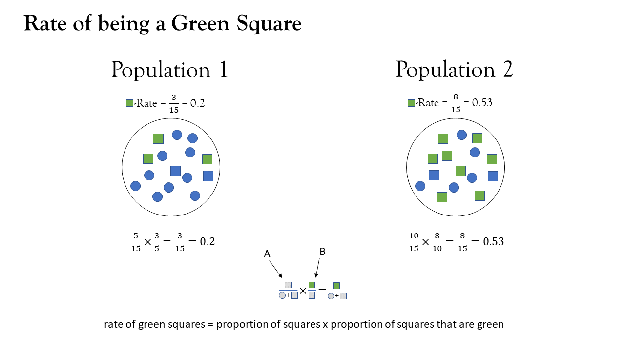
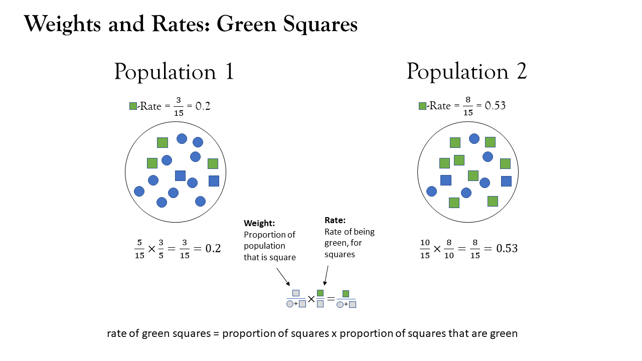
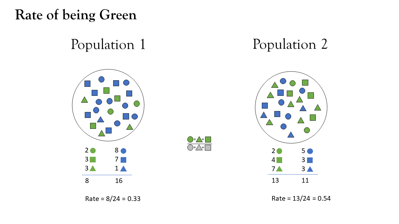
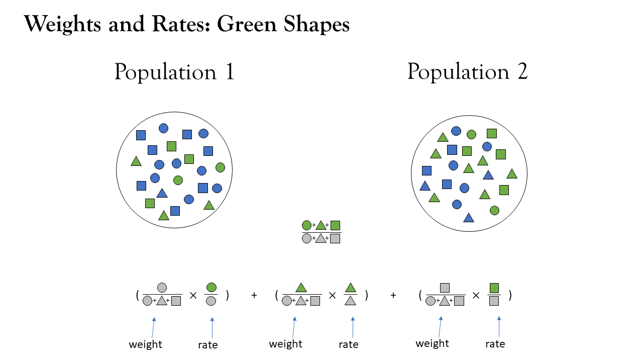
population structure
population share
relative size of sub group is another factor
\[ \text{Green Rate} = \sum\limits_{\text{shape }i} \frac{n_{i}}{n} \cdot \frac{green_{i}}{n_{i}} \]
decomposition within each sub-group?
separate out data into each subgroup
do decomposition of weight * rate on each subgroup
sum it all up
\[ \small \begin{align} W\text{-effect} = \,\,&(W_{2\,\bigcirc} - W_{1\,\bigcirc})\left( \frac{R_{1\,\bigcirc}+R_{2\,\bigcirc}}{2} \right) \\ &+ \\ &(W_{2\,\triangle} - W_{1\,\triangle})\left( \frac{R_{1\,\triangle}+R_{2\,\triangle}}{2} \right) \\ &+ \\ &(W_{2\,\square} - W_{1\,\square})\left( \frac{R_{1\,\square}+R_{2\,\square}}{2} \right) \\ \end{align} \]
What a lot of effort!
decomposition on vectors
do the decomposition of weight * rate, but instead of a single number, these are vectors.
\[ W\text{-effect} = \,\, (\vec{W}_{2} - \vec{W}_{1})\left( \frac{\vec{R}_{1}+\vec{R}_{2}}{2} \right) \] \[ \vec{W} = \begin{bmatrix} W_{\bigcirc} \\ W_{\triangle} \\ W_{\square} \end{bmatrix}, \vec{R} = \begin{bmatrix} R_{\bigcirc} \\ R_{\triangle} \\ R_{\square} \end{bmatrix}, \]
decomposition on vectors
Note we need to specify the ratefunction.
When weights and rates are vectors, then weight * rate will return a vector, but we need it to return a summary value, e.g., sum(weight * rate)
alternatively (or equivalently):
If we’re thinking about things in terms of population composition, then we can make use of:
id_vars: specify the variable(s) that define sub-groupscrossclassified: specify the variable that gives the sub-group size
With just one variable defining the sub-groups, this is (usually\(^*\)) just the same as the method on the slide previous
\(^*\)aside
population subgroup composition is a driver of the rate construction
decomposition of population rate with weights as a composite factor
\[
\sum\limits_i w_i \,\,\cdot a_i \,\cdot\, b_i \,\cdot\, c_i
\]
population subgroups are ‘containers’ for the rate
within-subgroup decomposition of rates, and decomposition of population rate as sum of weights*rates. \[ \sum\limits_i w_i \,\,\cdot \underset{\uparrow \atop a_i \cdot b_i \cdot c_i}{r_i} \]
“cross-classified”
sub-groups defined by multiple variables
combinations of age, sex, race, area, etc.
# A tibble: 12 × 5
     pop     i     j size  rate
   <int> <int> <int> <chr> <chr>
 1     1     1     1 n_11  r_11
 2     1     1     2 n_12  r_12
 3     1     1     3 n_13  r_13
 4     1     2     1 n_21  r_21
 5     1     2     2 n_22  r_22
 6     1     2     3 n_23  r_23
 7     2     1     1 n_11  r_11
 8     2     1     2 n_12  r_12
 9     2     1     3 n_13  r_13
10     2     2     1 n_21  r_21
11     2     2     2 n_22  r_22
12     2     2     3 n_23  r_23
# A tibble: 24 × 6
pop i j k size rate
<int> <int> <int> <int> <chr> <chr>
1 1 1 1 1 n_111 r_111
2 1 1 1 2 n_112 r_112
3 1 1 2 1 n_121 r_121
4 1 1 2 2 n_122 r_122
5 1 1 3 1 n_131 r_131
6 1 1 3 2 n_132 r_132
7 1 2 1 1 n_211 r_211
8 1 2 1 2 n_212 r_212
9 1 2 2 1 n_221 r_221
10 1 2 2 2 n_222 r_222
# ℹ 14 more rowsexample:
Code
eg5.3 <- tibble(
  pop = rep(c(1985, 1970), e = 22),
  age = rep(rep(1:11, 2), 2),
  race = rep(rep(1:2, e = 11), 2),
  # number of people in age-race-group
  size = c(
    3041, 11577, 27450, 32711, 35480, 27411, 19555, 19795, 15254, 8022,
    2472, 707, 2692, 6473, 6841, 6547, 4352, 3034, 2540, 1749, 804, 236,
    2968, 11484, 34614, 30992, 21983, 20314, 20928, 16897, 11339, 5720,
    1315, 535, 2162, 6120, 4781, 3096, 2718, 2363, 1767, 1149, 448, 117
  ),
  # death rate in age-race-group
  rate = c(
    9.163, 0.462, 0.248, 0.929, 1.084, 1.810, 4.715, 12.187, 27.728, 64.068, 157.570,
    17.208, 0.738, 0.328, 1.103, 2.045, 3.724, 8.052, 17.812, 34.128, 68.276, 125.161,
    18.469, 0.751, 0.391, 1.146, 1.287, 2.672, 6.636, 15.691, 34.723, 79.763, 176.837,
    36.993, 1.352,0.541, 2.040, 3.523, 6.746, 12.967, 24.471, 45.091, 74.902, 123.205
  )
)

eg5.3
# A tibble: 44 × 5
pop age race size rate
<dbl> <int> <int> <dbl> <dbl>
1 1985 1 1 3041 9.16
2 1985 2 1 11577 0.462
3 1985 3 1 27450 0.248
4 1985 4 1 32711 0.929
5 1985 5 1 35480 1.08
6 1985 6 1 27411 1.81
7 1985 7 1 19555 4.72
8 1985 8 1 19795 12.2
9 1985 9 1 15254 27.7
10 1985 10 1 8022 64.1
# ℹ 34 more rowscombined ij-mix contribution
Code
# A tibble: 44 × 7
pop age race size rate agerace agerace_w
<dbl> <int> <int> <dbl> <dbl> <fct> <dbl>
1 1985 1 1 3041 9.16 1.1 0.0127
2 1985 2 1 11577 0.462 2.1 0.0485
3 1985 3 1 27450 0.248 3.1 0.115
4 1985 4 1 32711 0.929 4.1 0.137
5 1985 5 1 35480 1.08 5.1 0.149
6 1985 6 1 27411 1.81 6.1 0.115
7 1985 7 1 19555 4.72 7.1 0.0819
8 1985 8 1 19795 12.2 8.1 0.0829
9 1985 9 1 15254 27.7 9.1 0.0639
10 1985 10 1 8022 64.1 10.1 0.0336
# ℹ 34 more rowsseparate i and j contributions?
ignoring the ij interaction.. (Don’t do this!!)
Code
# A tibble: 44 × 7
pop age race size rate age_w race_w
<dbl> <int> <int> <dbl> <dbl> <dbl> <dbl>
1 1985 1 1 3041 9.16 0.0157 0.849
2 1985 2 1 11577 0.462 0.0598 0.849
3 1985 3 1 27450 0.248 0.142 0.849
4 1985 4 1 32711 0.929 0.166 0.849
5 1985 5 1 35480 1.08 0.176 0.849
6 1985 6 1 27411 1.81 0.133 0.849
7 1985 7 1 19555 4.72 0.0946 0.849
8 1985 8 1 19795 12.2 0.0936 0.849
9 1985 9 1 15254 27.7 0.0712 0.849
10 1985 10 1 8022 64.1 0.0370 0.849
# ℹ 34 more rowsseparate i and j contributions
symetrically separating out ij interaction
# A tibble: 44 × 5
     pop   age  race  size   rate
   <dbl> <int> <int> <dbl>  <dbl>
 1  1985     1     1  3041  9.16
 2  1985     2     1 11577  0.462
 3  1985     3     1 27450  0.248
 4  1985     4     1 32711  0.929
 5  1985     5     1 35480  1.08
 6  1985     6     1 27411  1.81
 7  1985     7     1 19555  4.72
 8  1985     8     1 19795 12.2
 9  1985     9     1 15254 27.7
10  1985    10     1  8022 64.1
# ℹ 34 more rowsrequirements
exhaustive stratification - sub-groups should cover 100% of the population of interest.
both populations must have same subgroups
no subgroups of size zero
More than two populations?
example
Code
scbrth <-
  tribble(
    ~year, ~n_people, ~n_women, ~n_women1544, ~n_births,
    1991,   5083330,  2638815,      1121555,     67024,
    2000,   5062940,  2631014,      1079356,     53076,
    2010,   5262200,  2713982,      1058324,     58791,
  ) |>
  mutate(
    crude = n_births/n_people*1e3,
    propw = n_women/n_people,
    propw1544 = n_women1544/n_women,
    bpw = n_births/n_women1544*1e3
  )
scbrth
# A tibble: 3 × 9
year n_people n_women n_women1544 n_births crude propw propw1544 bpw
<dbl> <dbl> <dbl> <dbl> <dbl> <dbl> <dbl> <dbl> <dbl>
1 1991 5083330 2638815 1121555 67024 13.2 0.519 0.425 59.8
2 2000 5062940 2631014 1079356 53076 10.5 0.520 0.410 49.2
3 2010 5262200 2713982 1058324 58791 11.2 0.516 0.390 55.6a problem..
if we just look at pairwise decompositions..
           1991  2000     diff decomp
propw     11.82 11.83  0.01251  -0.46
propw1544 12.02 11.61 -0.41808  15.47
bpw       12.96 10.67 -2.29626  84.99
crude 13.19 10.48 -2.70182 100.00 2000 2010 diff decomp
propw 10.88 10.80 -0.08189 -11.88
propw1544 11.12 10.57 -0.55001 -79.82
bpw 10.19 11.51 1.32099 191.70
crude 10.48 11.17 0.68909 100.00We have multiple sets of standardised rates.
And internally inconsistent decomposition effects.
What we want:
\[\small
\begin{align}
\text{BPW-effect}_{\text{1991v2010}} &= \text{BPW-effect}_{\text{1991v2000}} + \\ & \quad \,\,\,\,\text{BPW-effect}_{\text{2000v2010}}
\end{align}
\]
What we have:
\[\small
\begin{align}
-0.88746 &\neq -2.29626 + 1.32099 \\
-0.88746 &\neq -0.9753 \,\,!?!?\\
\end{align}
\]
a solution
Averaging over different possible ways to achieve consistency through substituting in standardised rates for one another.
e.g.,:

In DasGuptR
It does it all for us:
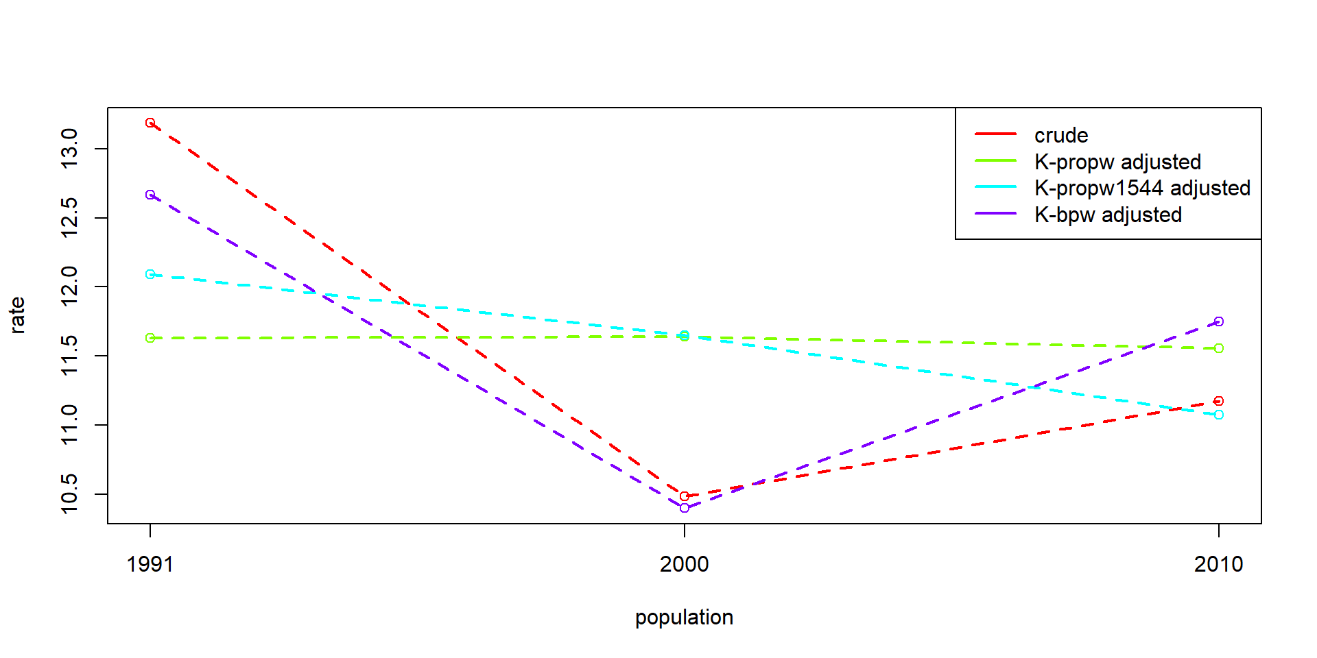
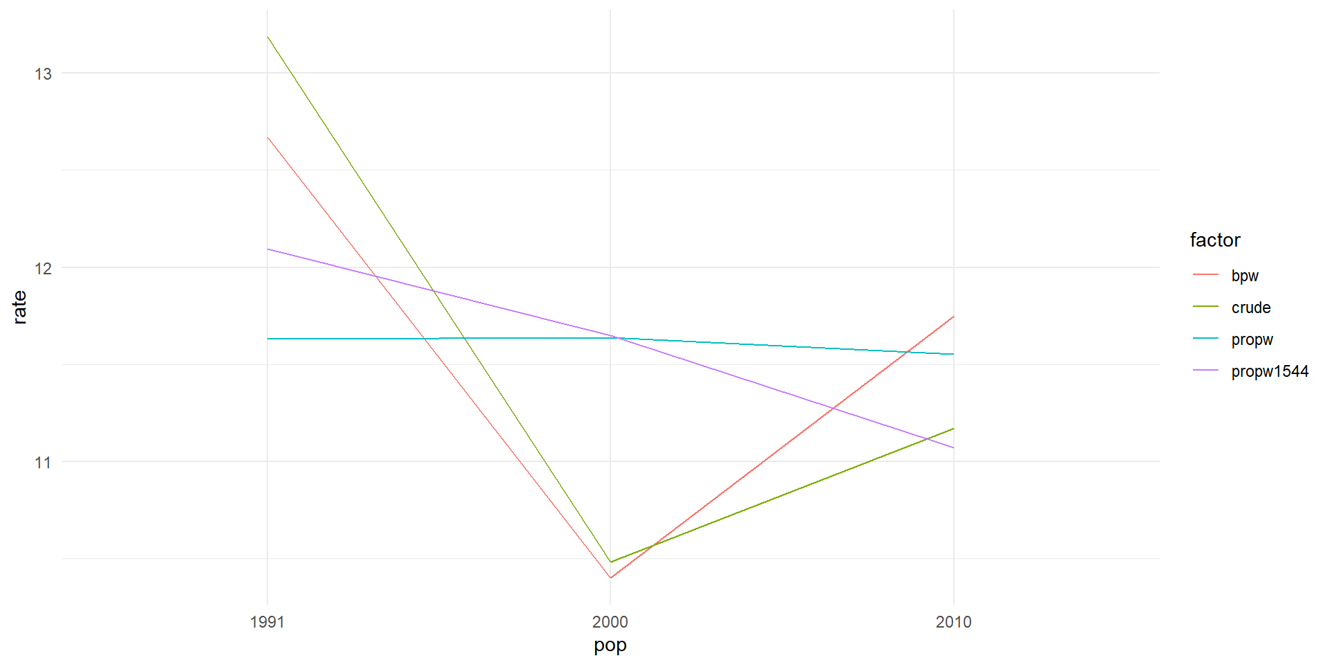
           1991  2000  2010
propw     11.63 11.64 11.55
propw1544 12.09 11.65 11.07
bpw       12.67 10.40 11.75
crude     13.19 10.48 11.17
Note we don’t get the decomposition effects unless we specify which pair of populations.
These are now based on standardisation across the full set.